In my previous post I wrote about generational cycles, which were identified by Neil Howe and William Strauss. However, cycles also appear in financial markets. Have you heard of legendary investors from the 19th and early 20th century that allegedly predicted financial booms and busts of the following 100 years? In the following I am going to take a closer look some of these investors and the predictions they made.
Samuel Benner
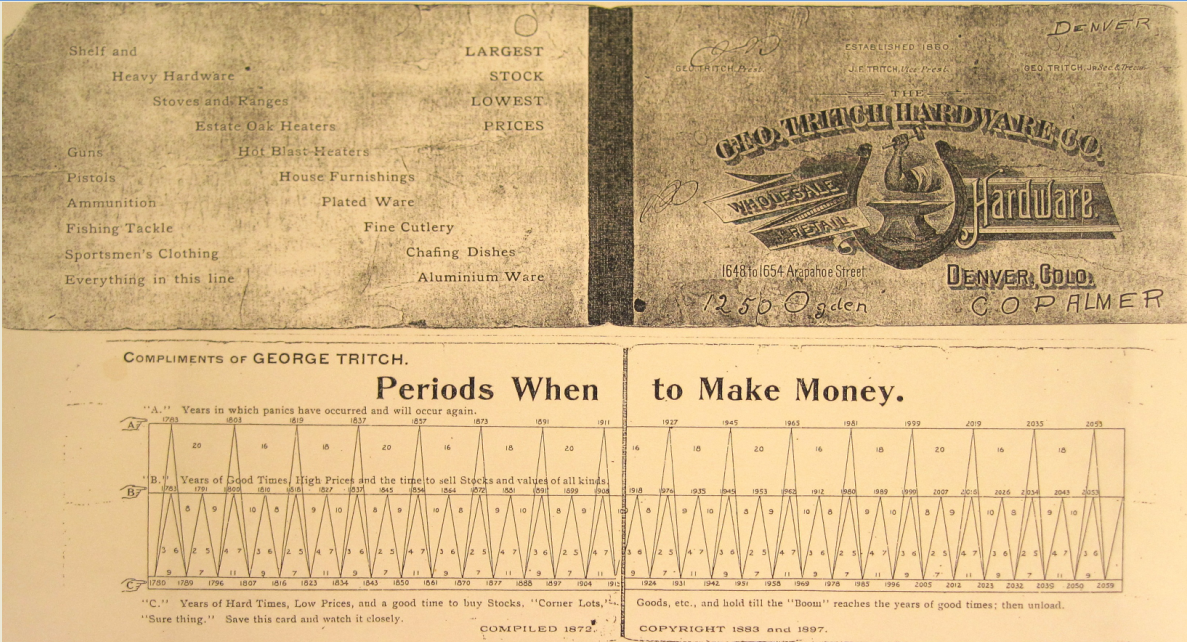
Samuel Benner was a prosperous farmer who was wiped out financially by the 1873 panic. When he tried to discern the causes of fluctuations in markets, he came across a large degree of cyclicality. The Benner Cycle is based on a major 54 year cycle. Market tops form in a recurring cylce of 16, 18 and 20 – leading to an average of 18 years. Benner also identified a 27 year cycle in pig iron prices with lows every 11, 9, 7 years and peaks in the order 8, 9, 10 years.
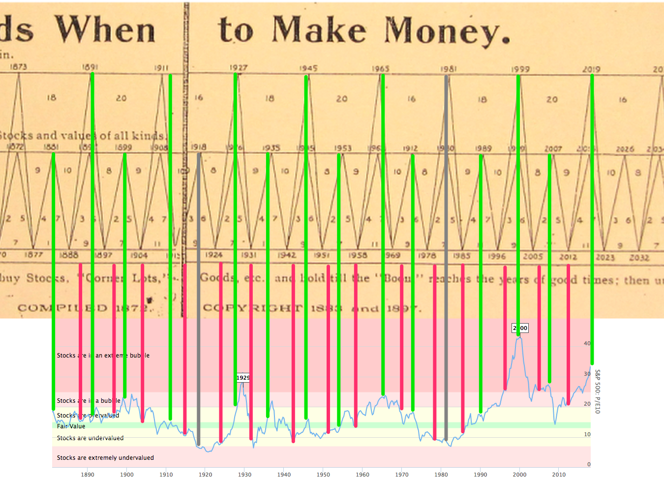
Benner eventually published the following chart in 1875 (!).
The table predicted panics (or highs respectively) for 1911, 1927, 1945, 1965, 1981, 1999, and 2019. Except for 1981, these were all good years to sell stocks. An overlay with the Shiller Price Earnings Ratio illustrates this fact. (Please note that the the two charts have slightly different time scales. The lines actually represent the years of the Benner cycle, even though they appear to be slightly off)
William Delbert Gann
The following table is infamous among traders. In 1909, William Delbert Gann reportedly constructed this legendary Financial Timetable providing a road map for the direction of US stock prices for the entire 20th century.
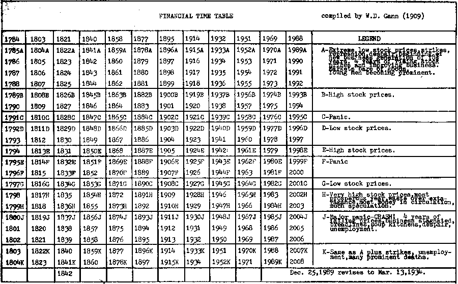
The table was calculated using the North Node lunar time cycle of 18.61 years (similar to Benner’s 18 years). To mimic the lunar declination cycle Gann simply alternated a sequence of +19, +18, +19, +18 etc.-years across the top to get an average length of 18.6-years. However, he noted that an adjustment would finally be due for Dec 25th, 1989.
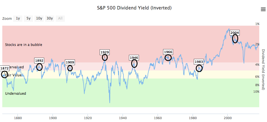
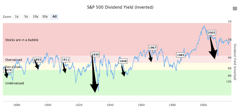
The H row predicts “very high stock prices”. The S&P 500 dividend yield is a valuation metric for the stock market and when we examine the years in row H on the dividend yield we see that these years accurately predicted market tops (notably 1929, 1946, and 1966):
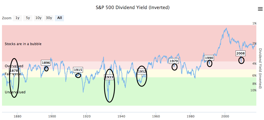
Note that the next row J predicts “Major Panic-CRASH! 4-years of falling prices”. Once again when we put these numbers on the S&P 500 dividend yield Gann’s predictions proved to be right:
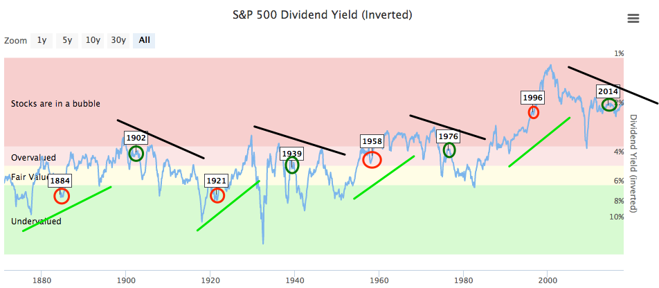
After these 4 years we reach the A row with “Extreme low stock prices”. Putting the years of row A into S&P 500 dividend yield gives us the following picture:
The C row does not produce such clean and obvious patterns. It simply stands for “Panic”. When we examine these years on the S&P 500 dividend yield we appear to get alternating highs and lows in alternating secular up- and down-trends.
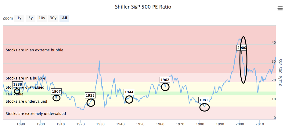
The F row also predicts years of “Panic”. When we put these years in the Shiller Price Earnings ratio we see that these years predicted lows in the stock market but also the turning of interest rates in 1981 and the bust of the 2000 Dot-com bubble.
Of course, Gann’s table can be extended into the future. The following Excel table accounts for the mentioned necessary adjustment (by adding one year to the cycle – see yellow mark) and extends Gann’s table until the year 2100. (I found another version that adds 2 years instead of one but I can’t find a reason why they would do that)
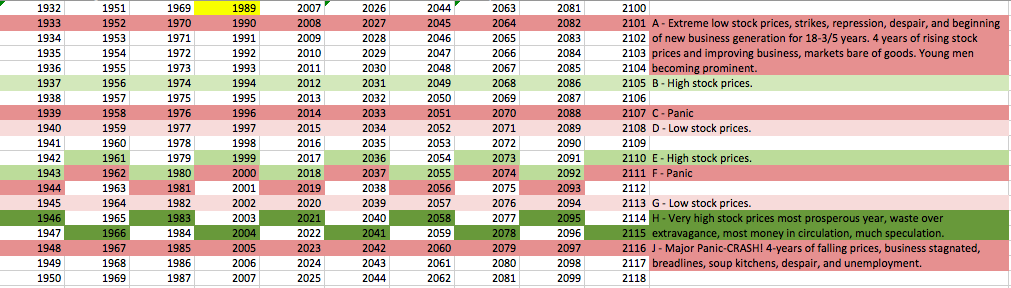
Just like the Benner cycle, the extended Gann table predicts high stock prices and a following panic in 2018 and 2019.
Final Thoughts
In an attempt to explain Benner’s accurate predictions Businessinsider writes “It makes some degree of intuitive sense that a farmer would recognize longer term cycles. Their entire year is based on the annual sowing/growing/reaping cycle; The 11 year solar cycle would certainly impact their crop yields, revenue, etc. So looking at how the variants of crop yield and prices impacts the overall economy and markets makes lots of sense.”
In the end, the cause for these accurate predictions and for cycles in financial markets might be multifaceted. It might include influences from the climate (which affect commodity prices), the generational cycle, the short-term business cycle (with economic expansions and recessions), and the longer-term debt cycle. No matter the cause, the cycles actually do appear in the data, which gives us the opportunity to learn from them and to anticipate the future.